Working with Bonds • fcaR

Introduction

In Formal Concept Analysis (FCA), a bond between two formal contexts $K_1 = (G_1, M_1, I_1)$ and $K_2 = (G_2, M_2, I_2)$ is a relation $R \subseteq G_1 \times M_2$ such that: - For every object $g \in G_1$ , the set of attributes $\{m \in M_2 \mid (g, m) \in R\}$ is an intent of $K_2$ . - For every attribute $m \in M_2$ , the set of objects $\{g \in G_1 \mid (g, m) \in R\}$ is an extent of $K_1$ .

Bonds represent “compatible” relations between the objects of one context and the attributes of another. Mathematically, the set of all bonds between two contexts, ordered by inclusion, forms a complete lattice called the Bond Lattice.

In fcaR, bonds are treated as first-class citizens with a dedicated BondLattice class that extends the standard ConceptLattice.

library(fcaR)

Computing Bonds

The main function to compute bonds is bonds(). It takes two FormalContext objects as input.

To keep this example fast, we will generate two small random formal contexts ( $4 \times 4$ ).

set.seed(42)
# Context 1
mat1 <- matrix(sample(0:1, 16, replace = TRUE), nrow = 4, ncol = 4)
rownames(mat1) <- paste0("O", 1:4)
colnames(mat1) <- paste0("A", 1:4)
fc1 <- FormalContext$new(mat1)

# Context 2
mat2 <- matrix(sample(0:1, 16, replace = TRUE), nrow = 4, ncol = 4)
rownames(mat2) <- paste0("P", 1:4)
colnames(mat2) <- paste0("B", 1:4)
fc2 <- FormalContext$new(mat2)

To compute the bond lattice:

bl <- bonds(fc1, fc2, method = "conexp")
bl
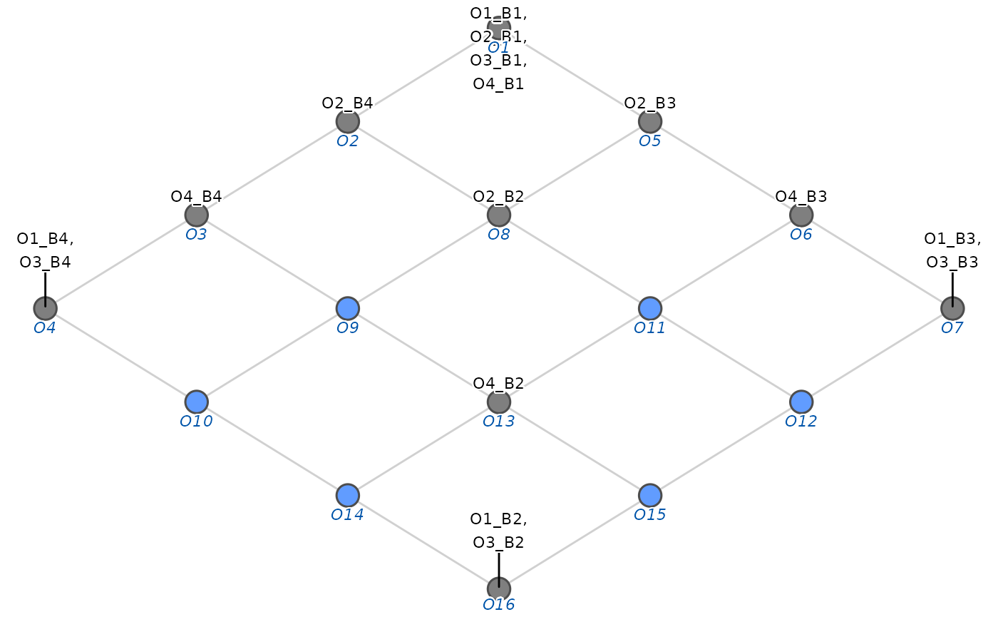
#> Bond Lattice between two formal contexts:
#> - Context 1 (G1): 4 objects (O1, O2...)
#> - Context 2 (M2): 4 attributes (B1, B2...)
#> - Total Bonds: 16

Computation Methods

The bonds() function provides two optimized C++ methods: 1. "conexp" (Default): Uses an implication-based approach on a tensor product of the contexts. It is generally the fastest for dense or moderately sized contexts. 2. "mcis": A backtracking algorithm that operates directly on the pre-computed concept sets of both contexts. It can be more efficient in specific structural configurations.

# Using the backtracking method
bl_mcis <- bonds(fc1, fc2, method = "mcis")
bl_mcis$size()
#> [1] 16

The BondLattice Object

The result of bonds() is an object of class BondLattice. Since this class inherits from ConceptLattice, you can use all standard lattice operations.

Visualization

You can plot the Hasse diagram of the bond lattice:

bl$plot()

Extracting Bonds

Each node in the bond lattice represents a specific bond (a relation). You can extract these relations as individual FormalContext objects:

# Get all bonds as a list of FormalContexts
all_bonds <- bl$get_bonds()
length(all_bonds)
#> [1] 16

# Inspect the first non-trivial bond
# (Note: Bond 1 is usually the "Core" or minimal bond)
all_bonds[[1]]
#> FormalContext with 4 objects and 4 attributes.
#>     B1  B2  B3  B4  
#>  O1  X              
#>  O2  X              
#>  O3  X              
#>  O4  X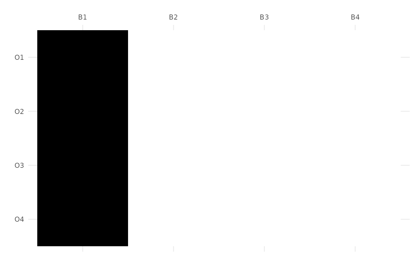

The Core Bond

The “Core” bond is the intersection of all bonds (the infimum of the lattice). It represents the most fundamental consensus between the two contexts.

core <- bl$get_core()
core$plot()

Verifying Bonds

If you have a relation (as a matrix or a FormalContext) and want to check if it satisfies the mathematical definition of a bond between two contexts:

# Take an existing bond and check it
mat_bond <- methods::as(all_bonds[[1]]$incidence(), "matrix")
is_bond(fc1, fc2, mat_bond)
#> [1] TRUE

# Check an arbitrary (likely invalid) relation
random_rel <- matrix(0, nrow = nrow(mat_bond), ncol = ncol(mat_bond))
is_bond(fc1, fc2, random_rel)
#> [1] FALSE

Similarity and Complexity Metrics

The BondLattice class provides a similarity() method to compute various metrics that describe the relationship between the two formal contexts.

# 1. Logical Affinity (Log-Bond)
# Measures how much the two contexts share a common logical structure.
# 1.0 means perfect affinity.
bl$similarity("log-bond")
#> [1] 0.9620358

# 2. Structural Complexity
# Ratio of irreducible bonds to total bonds. 
# Lower values indicate more emergent structural properties.
bl$similarity("complexity")
#> [1] 0.375

# 3. Core Agreement
# Ratio of filled cells in the Core bond versus the Top (largest) bond.
bl$similarity("core-agreement")
#> [1] 0.25

# 4. Interaction Entropy
# Based on the log-size of the lattices.
bl$similarity("entropy")
#> [1] 0.4806578

Order-Theoretic Properties

Bonds also allow exploring deep structural properties of the interaction between contexts using measures like Width and Dimension.

Dilworth’s Width: The size of the largest antichain in the bond lattice.
Order Dimension: The minimum number of linear orders whose intersection is the bond lattice.

# Dilworth's Width
bl$similarity("width")
#> [1] 4

# Order Dimension (estimated via heuristic)
bl$similarity("dimension")
#> [1] 2

These measures can also be expressed as indices normalized by the lattice size:

bl$similarity("width-index")
#> [1] 0.25
bl$similarity("dimension-index")
#> [1] 0.5

Summary

Bonds provide a powerful mathematical framework to analyze the alignment or interaction between different perspectives (contexts) on the same objects or attributes. With fcaR, you can efficiently calculate large bond lattices, visualize them, and extract meaningful metrics to quantify context similarity and structural emergence.